Robust Geodesic Regression

Ronny Bergmann 2026-07-04

Prequel

This notebook reproduces the results and images of Section 6.1 in [BB26]. We use the following packages and parameters

using Colors, Distributions, GeometryBasics, GLMakie, Makie, ManifoldDiff, Manifolds, Manopt, NamedColors, Random, RecursiveArrayTools
## Set the interval we sample the points from on the geodesic
T = 1.0
## Number of points along the geodesic on [-T,T]
N = 100
## Outlier parameters
### Distance the outliers are moved
r = π / 4
### Number of outliers per each segment
oN = 7
## And set these slightly asymmetric
outlier_indices = [4:(4 + oN - 1)..., [(N - 11):-1:(N - 11 - oN + 1)...]...];
## Plotting colors
ptc = NamedColors.load_paul_tol()
orig_color = ptc["mutedcyan"]
noisy_color = ptc["mutedpurple"]
lsq_color = ptc["mutedsand"]
robust_color = ptc["mutedgreen"]

Introduction

For robust geodesic regression on a Riemannian manifolds $\mathcal M$ consider $m \in \mathbb N$ points $q_1,\ldots,q_m \in \mathcal M$ thereon associated to scalar values $t_1,\ldots,t_m \in \mathbb R$. We further denote the geodesic starting in a point $p \in \mathcal M$ in direction $X \in T_p\mathcal M$ by The task of geodesic regression is given as the problem on the tangent bundle $T\mathcal M$ to find the geodesic $\gamma_{p,X}$, i.e. both $p$ and $X$, that “best fits” the data with $\gamma_{p,X}(t_i) \approx q_i$, $i=1,\ldots,m$, where we still have the freedom to choose in what sense we mean to address the approximately equal condition. We consider

\[\operatorname*{argmin}_{(p,X) \in T\mathcal M} \sum_{i=1}^m \rho\bigl( d_{\mathcal M}^2( \gamma_{p,X}(t_i), q_i) \bigr),\]

where $\rho$ is a robustifier applied to every summand. Choosing $\rho(x) = x$ we get the classical (least squares) geodesic regression [Fle13]. Here we want to consider approximations of the case where $\rho(x) = \sqrt{x}$, where the sum reduces to the sum of distances or the robust geodesic regression. Since that is no longer differentiable, we use a scaled version of the Huber robustifier.

Setup

We first setup the manifold, the true point, tangent vector, and data

S = Manifolds.Sphere(2)
M = TangentBundle(S)

and the original data as

p_true = [0.0, 1.0, 0.0]
X_true = π / 2 .* [1.0, 0.0, 1.0]
ts_true = collect(range(; start = -T, stop = T, length = N))
qs_true = geodesic(S, p_true, X_true, ts_true)
geo_line = geodesic(S, p_true, X_true, range(-T, T; length = 1000))

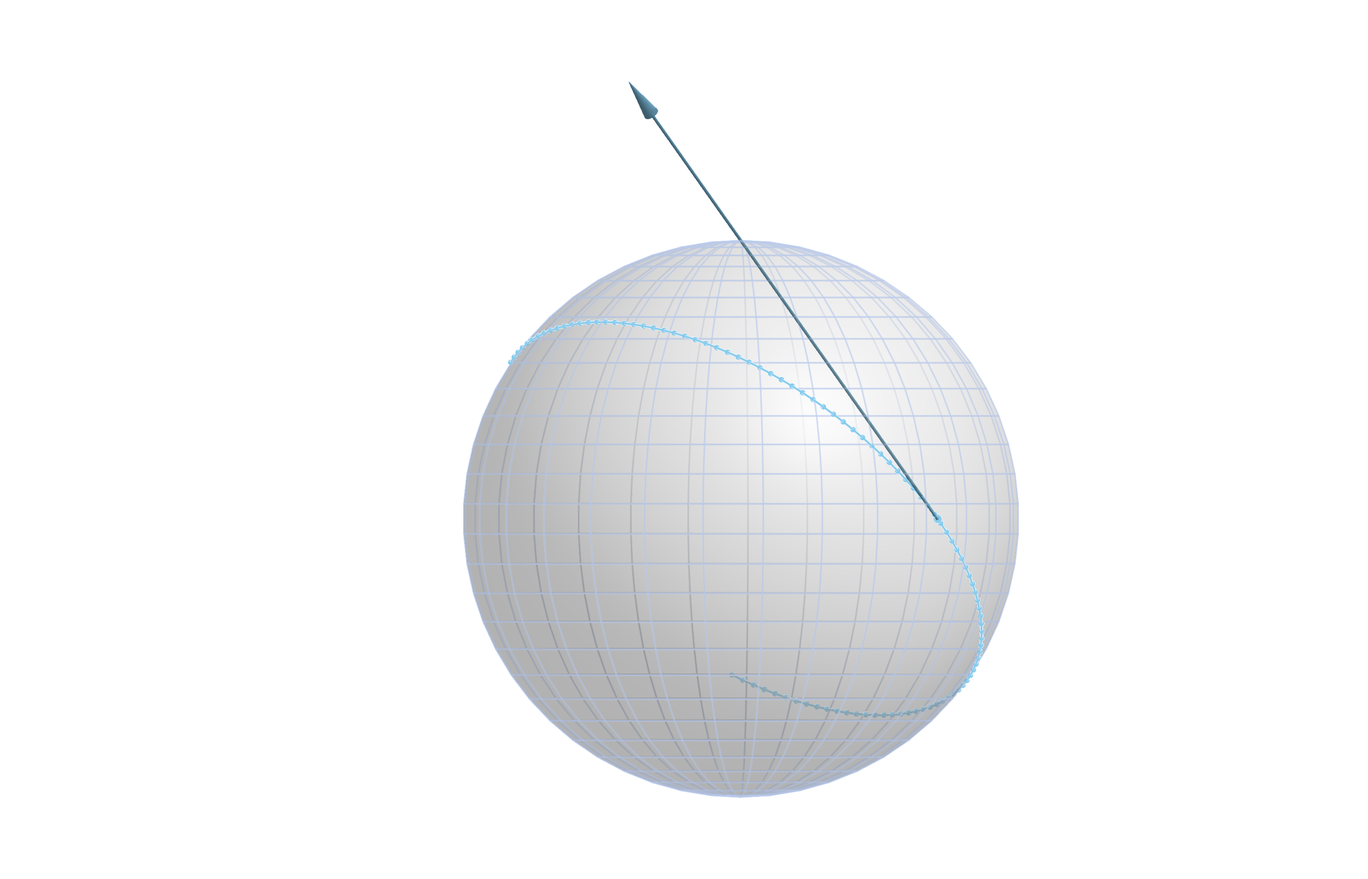
which looks like

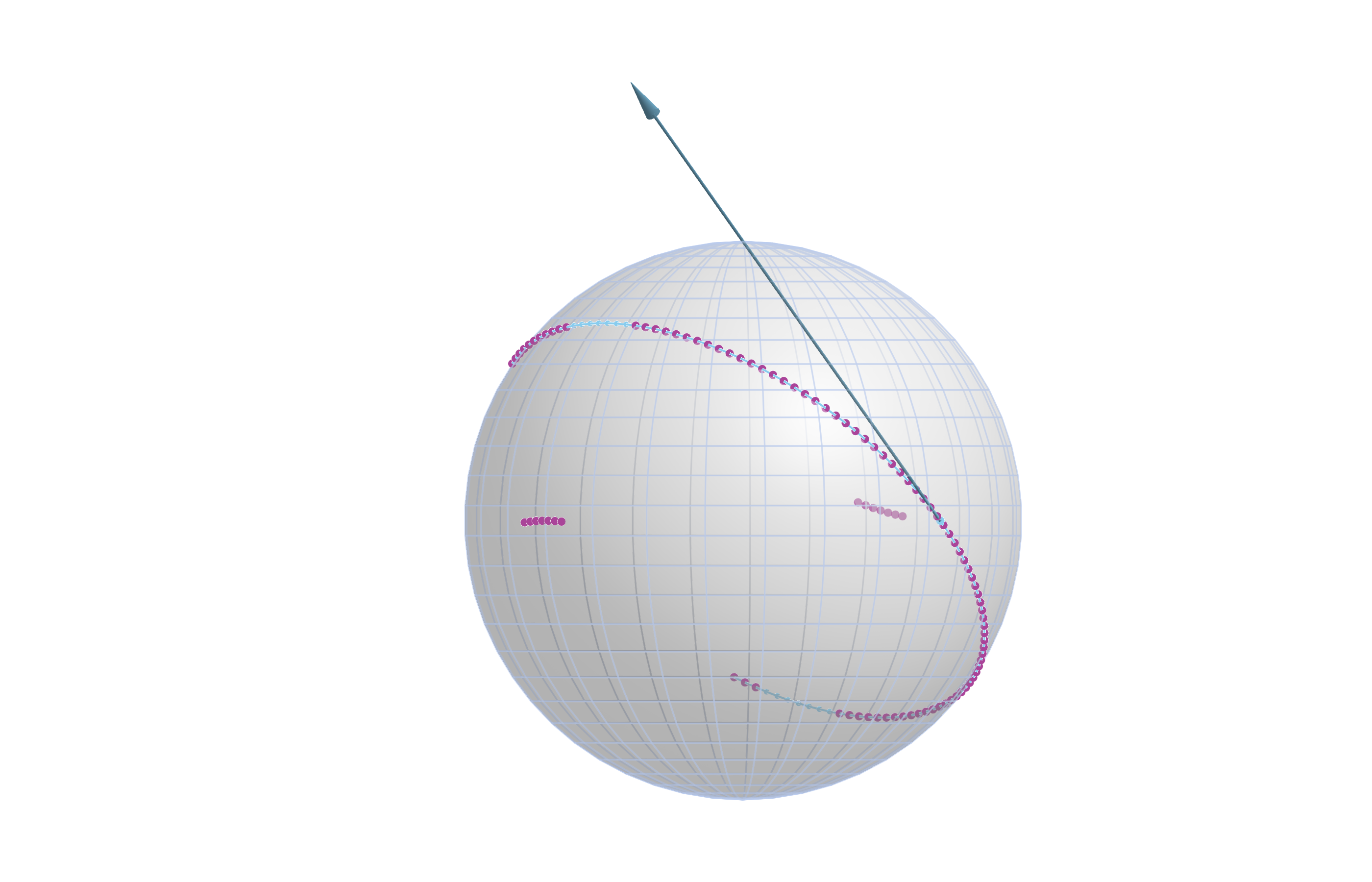
We then generate outliers

Random.seed!(42)
R(α) = [cos(α) -sin(α); sin(α) cos(α)]
data = [
  if i ∈ outlier_indices
    # all are outliers to the left or right
    α = π / 2
    c = get_coordinates(S, q, parallel_transport_to(S, p_true, X_true, q), DefaultOrthonormalBasis())
    X_offset = get_vector(S, q, r / norm(c) .* R(α) * c, DefaultOrthonormalBasis())
    exp(S, q, X_offset)
  else
    q
  end
  for (i, q) in enumerate(qs_true)
]

The Residual and its Jacobian

We first define the overall least squares cost as well as its partial gradients w. r. t. p and X for a single summand

function cost1(M::AbstractManifold, p, X, ti::Real, di)
    return 1 / 2 * distance(M, exp(M, p, ti * X), di)^2
end
function cost1_grad_p(M::AbstractManifold, p, X, ti::Real, di)
    z = exp(M, p, ti * X)
    gz = ManifoldDiff.grad_distance(M, di, z, 1)
    return ManifoldDiff.adjoint_differential_exp_basepoint(M, p, ti * X, gz)
end
function cost1_grad_X(M::AbstractManifold, p, X, ti::Real, di)
    z = exp(M, p, ti * X)
    gz = ManifoldDiff.grad_distance(M, di, z, 1)
    return ti * ManifoldDiff.adjoint_differential_exp_argument(M, p, ti * X, gz)
end

This is then used to define the overall residual F and its Jacobian JF.

function F(M, P; t = ts_true, d = data)
    # Extract manifold and (p,X)
    S = base_manifold(M); p = P[M, :point]; X = P[M, :vector]
    return [distance(S, geodesic(S, p, X, ti), di) for (ti, di) in zip(t, d)]
end
function JF(M, P; t = ts_true, d = data)
  # Extract manifold and (p,X)
  S = base_manifold(M); p = P[M, :point]; X = P[M, :vector]
  return [
    ArrayPartition(
      cost1_grad_p(S, p, X, ti, di), cost1_grad_X(S, p, X, ti, di),
    )
    for (ti, di) in zip(t, d)
  ]
end

We combine these into a VectorGradientFunction

f = VectorGradientFunction(
    F, JF, N;
    evaluation = AllocatingEvaluation(),
    function_type = FunctionVectorialType(),
    jacobian_type = FunctionVectorialType(),
)

And we set a start point p0.

m = mean(S, data)
X0 = log(S, m, data[end])
p0 = ArrayPartition(m, X0)

Least Squares Geodesic Regression

We first run the LevenbergMarquardt solver without a robustifier, which means we solver the least squares problem, or in other words set $\rho(x) = x$

P_star = LevenbergMarquardt(
    M, f, p0;
    damping_increase_factor = 2.0, candidate_acceptance_threshold = 0.2, damping_term_min = 1.0e-5,
    damping_increase_threshold = 0.2,
    damping_reduction_threshold = 0.5,
    scaling_threshold = 1.0e-1, scaling_mode = :Strict,
    retraction_method = StabilizedRetraction(default_retraction_method(M)),
    debug = [:Iteration, (:Cost, "f(x): %8.8e "), :damping_term, "\n",
    10, :Stop],
)

And we can extract the minimizer parts $P^* = (p^*,X^*)$ as

p_star = P_star[M, :point]
X_star = P_star[M, :vector]
qs_star = geodesic(S, p_star, X_star, ts_true)
geo_line_mean = geodesic(S, p_star, X_star, range(-T, T; length = 1000))

which yields the result

scatterlines!(
  ax1, Point3d.(geo_line_mean); markersize = 0, color = lsq_color, linewidth = 2,
)
scatter!(ax1, Point3d.([p_star]); markersize = 12, color = lsq_color)
scatter!(ax1, Point3d.(qs_star); markersize = 8, color = lsq_color)
arrows3d!(
  ax1, Point3d.([p_star]), Point3d.([X_star]);
  color = lsq_color, transparency = true, shaftradius = 0.0025, tiplength = 0.075, tipradius = 0.0125,
)
fig1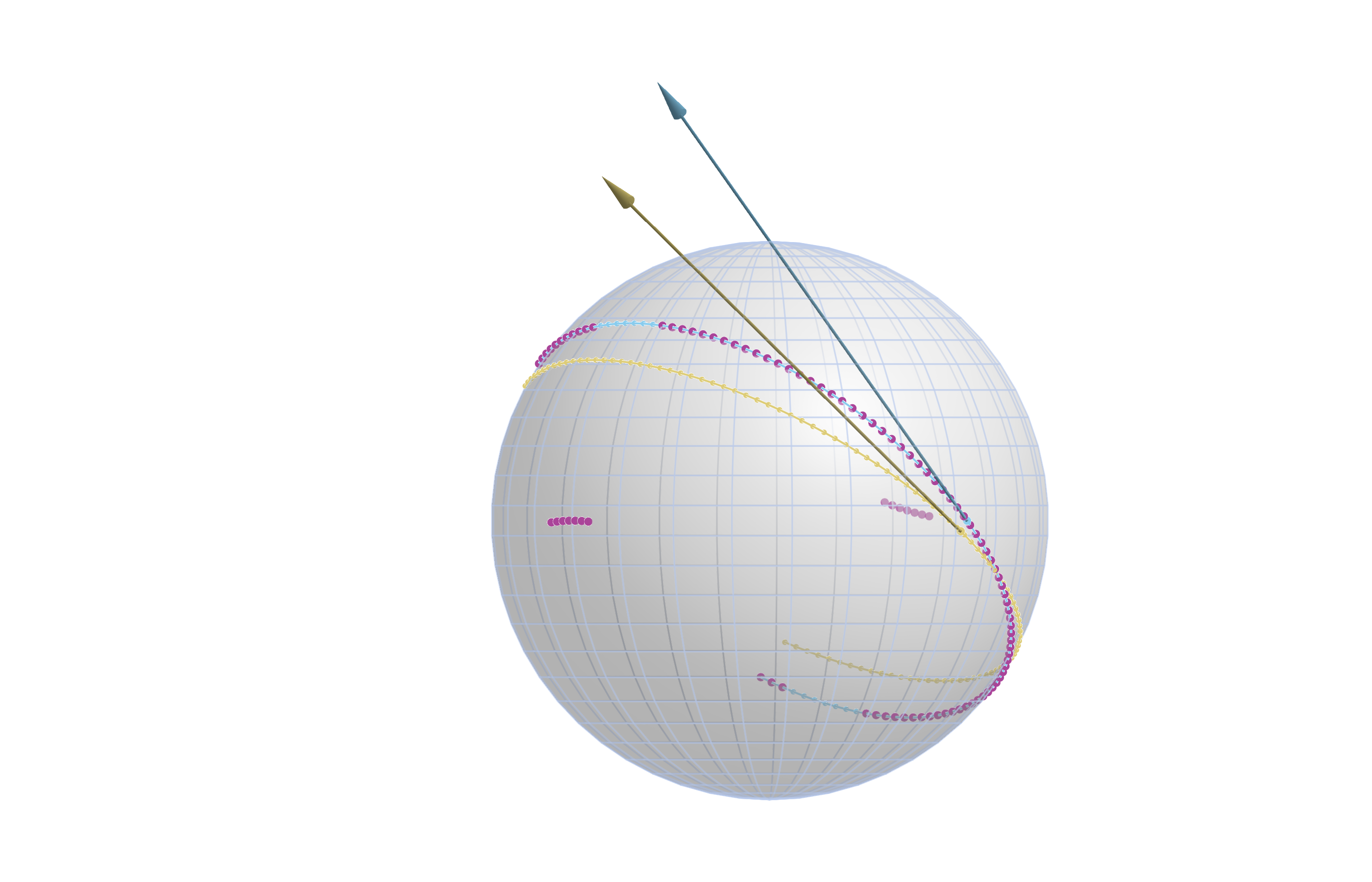

One can see, that the outliers yield that the least squares result is slightly “skewed” to one side.

Robust Geodesic Regression

As comparison we take a scaled version of the HuberRobustifier by concatenting it with a scaling, so that we move the “cutoff” to a value 1.0e-4, see ScaledRobustifierFunction.

The solver call uses the same variables for the remaining setup than the previous run.

P_ast = LevenbergMarquardt(
  M, f, p0;
  damping_increase_factor = 8.0, candidate_acceptance_threshold = 0.2, damping_term_min = 1.0e-5,
  scaling_threshold = 1.0e-1, scaling_mode = :Strict,
  damping_increase_threshold = 0.2,
  damping_reduction_threshold = 0.5,
  robustifier = 1.0e-4 ∘ HuberRobustifier(),
  retraction_method = StabilizedRetraction(default_retraction_method(M)),
  debug = [:Iteration, (:Cost, "f(x): %8.8e "), :damping_term, "\n", 10, :Stop],
)

And we again extract the minimizer parts

p_ast = P_ast[M, :point]
X_ast = P_ast[M, :vector]
qs_ast = geodesic(S, p_ast, X_ast, ts_true)
geo_line_robust = geodesic(S, p_ast, X_ast, range(-T, T; length = 1000))

to add them to the figure

scatterlines!(
  ax1, Point3d.(geo_line_robust); markersize = 0, color = robust_color, linewidth = 2,
)
scatter!(ax1, Point3d.([p_ast]); markersize = 12, color = robust_color)
scatter!(ax1, Point3d.(qs_ast); markersize = 8, color = robust_color)
arrows3d!(
  ax1, Point3d.([p_ast]), Point3d.([X_ast]);
  color = robust_color, transparency = true, shaftradius = 0.0025, tiplength = 0.075, tipradius = 0.0125,
)
fig1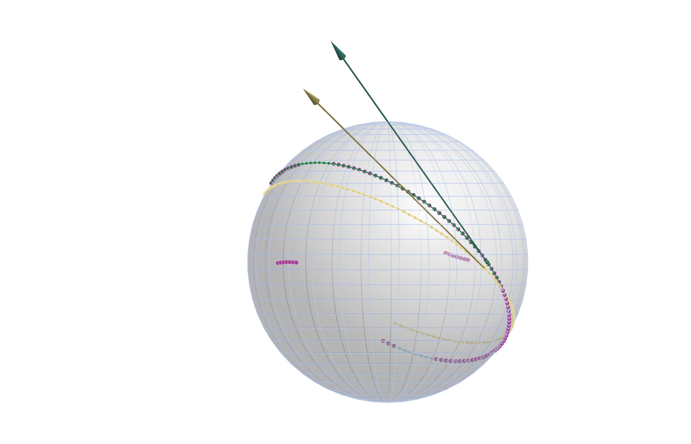

Here the new (green) dots and the tangent vector lie exactly on the original geodesic visually.

If we measure the (mean) error we get for least squares

1 / N * norm([distance(S, qi, qmi) for (qi, qmi) in zip(qs_true, qs_star)])

0.013904282413539831

On the other hand for the robust case we get

1 / N * norm([distance(S, qi, qmi) for (qi, qmi) in zip(qs_true, qs_ast)])

2.2737844213842437e-6

Literature

Status `~/Repositories/Julia/ManoptExamples.jl/examples/Project.toml`
  [6e4b80f9] BenchmarkTools v1.8.0
  [336ed68f] CSV v0.10.16
  [13f3f980] CairoMakie v0.15.12
  [0ca39b1e] Chairmarks v1.3.1
  [35d6a980] ColorSchemes v3.31.0
  [5ae59095] Colors v0.13.1
  [a93c6f00] DataFrames v1.8.2
  [31c24e10] Distributions v0.25.129
  [e9467ef8] GLMakie v0.13.12
  [5c1252a2] GeometryBasics v0.5.11
  [4d00f742] GeometryTypes v0.8.5
  [7073ff75] IJulia v1.34.4
  [682c06a0] JSON v1.6.1
  [8ac3fa9e] LRUCache v1.6.2
  [b964fa9f] LaTeXStrings v1.4.0
  [d3d80556] LineSearches v7.7.1
  [ee78f7c6] Makie v0.24.12
  [7351309b] ManifoldAsymptote v0.1.0
  [af67fdf4] ManifoldDiff v0.4.5
  [9d80ff41] ManifoldMakie v0.1.2
  [1cead3c2] Manifolds v0.11.28
  [3362f125] ManifoldsBase v2.4.0
⌃ [0fc0a36d] Manopt v0.6.0
  [5b8d5e80] ManoptExamples v0.1.18 `..`
  [51fcb6bd] NamedColors v0.2.3
  [6fe1bfb0] OffsetArrays v1.17.0
  [91a5bcdd] Plots v1.41.6
⌃ [08abe8d2] PrettyTables v3.3.2
  [6099a3de] PythonCall v0.9.35
  [f468eda6] QuadraticModels v0.9.16
  [731186ca] RecursiveArrayTools v4.3.2
  [1e40b3f8] RipQP v0.7.0
Info Packages marked with ⌃ have new versions available and may be upgradable.