The Constrained mean on high-dimensional Hyperbolic space.

Hajg Jasa, Ronny Bergmann 2026-04-06

Introduction

This example is to be thought of as a continuation of the Constrained Mean on Hyperbolic Space, where we compare the Intrinsic Convex Riemannian Proximal Gradient Method (CRPG) from [BJJP25a] with the Projected Gradient Algorithm (PGA) as introduced in [BFNZ25]. For CRPG, we test performances of both constant and backtracked stepsize strategies. This example reproduces the results from [BJJP25a], Section 6.4.

using Chairmarks, CSV, DataFrames, Manifolds, Manopt, CairoMakie, Random
import ColorSchemes.tol_vibrant

Consider the constrained Riemannian center of mass for a given set of points $q_i \in \mathcal M$, $i=1,\ldots,N$ given by

\[\operatorname*{arg\,min}_{p\in\mathcal C} \sum_{i=1}^N d_{\mathrm{M}}^2(p,q_i)\]

constrained to a set $\mathcal C \subset \mathcal M$.

The same problem can be formulated as an unconstrained optimization problem by introducing the characteristic function for the set $\mathcal C$:

\[\operatorname*{arg\,min}_{p\in\mathcal M} \sum_{i=1}^N d_{\mathrm{M}}^2(p,q_i) + \chi_{\mathcal C}(p)\]

where $\chi_{\mathcal C}(p) = 0$ if $p \in \mathcal C$ and $\chi_{\mathcal C}(p) = \infty$ otherwise. This formulation allows us to use CRPG to solve the problem.

For this experiment set $\mathcal M = \mathbb H^d$ for $d=2,\ldots,200$, the Hyperbolic space and the constrained set $\mathcal C = C_{c,r}$ as the ball of radius $r$ around the center point $c$, where we choose here $r=\frac{1}{\sqrt{n}}$ and $c = (0,\ldots,0,1)^{\mathrm{T}}$ and a $σ = \frac{3}{2}n^{1/4}$.

n_range = Vector(2:200)
radius_range = [1 / sqrt(n) for n ∈ n_range]
N_range = [400 for n ∈ n_range]
M_range = [Hyperbolic(n) for n ∈ n_range]
σ_range = [ 1.5/sqrt(sqrt(n-1)) for n ∈ n_range]
tol = 1e-7

The data consists of $N=200$ points, where we skew the data a bit to force the mean to be outside of the constrained set $\mathcal C$.

Cost, gradient and projection

We can formulate the constrained problem above in two different forms. Both share a cost and require a gradient. For performance reasons, we also provide a mutating variant of the gradient

f(M, p; pts=[]) = 1 / (2 * length(pts)) .* sum(distance(M, p, q)^2 for q in pts)

grad_f(M, p; pts=[]) = -1 / length(pts) .* sum(log(M, p, q) for q in pts)

function grad_f!(M, X, p; pts=[])
    zero_vector!(M, X, p)
    Y = zero_vector(M, p)
    for q in pts
        log!(M, Y, p, q)
        X .+= Y
    end
    X .*= -1 / length(pts)
    return X
end

We can model the constraint either with an inequality constraint $g(p) \geq 0$ or using a projection onto the set. For the gradient of $g$ and the projection we again also provide mutating variants. Lastly, we define the cost function $F$ as the sum of the original cost and the characteristic function for the set $\mathcal C$.

g(M, p; op=[], radius=1) = distance(M, op, p)^2 - radius^2;
# The characteristic function for the set C is defined with tol^2 to avoid numerical issues
characteristic_C(M, p; op=[], radius=1) = (g(M, p; op=op, radius=radius) ≤ tol^2) ? 0 : Inf;

function project_C(M, p; op=[], radius=1)
    X = log(M, op, p)
    n = norm(M, op, X)
    q = (n > radius) ? exp(M, op, (radius / n) * X) : copy(M, p)
    return q
end;

function project_C!(M, q, p; radius=1, op=[], X=zero_vector(M, op))
    log!(M, X, op, p)
    n = norm(M, op, X)
    if (n > radius)
        exp!(M, q, op, (radius / n) * X)
    else
        copyto!(M, q, p)
    end
    return q
end;

grad_g(M, p; op=[]) = -2 * log(M, p, op)
function grad_g!(M, X, p; op=[])
    log!(M, X, p, op)
    X .*= -2
    return X
end

F(M, p; pts=[], radius=1, op=[]) = f(M, p; pts=pts) + characteristic_C(M, p; op=op, radius=radius)

The mean

For comparison, we first compute the Riemannian center of mass, that is the minimization above but not constrained to $\mathcal C$. We can then project this onto $\mathcal C$. For the projected mean we obtain $g(p) = 0$ since the original mean is outside of the set, the projected one lies on the boundary.

We first generate all data

centers = [[zeros(n)..., 1.0] for n in n_range]
begin
    Random.seed!(5)
    data = [
        [
            exp(
                M,
                c,
                get_vector(
                    M, c, σ * randn(n) .+ 2 * r .* ones(n), DefaultOrthonormalBasis()
                ),
            ) for _ in 1:N
        ] for
        (c, r, n, N, M, σ) in zip(centers, radius_range, n_range, N_range, M_range, σ_range)
    ]
end

means = [mean(M, d) for (M, d) in zip(M_range, data)]
dc = [
    characteristic_C(M, m; op=c, radius=r) for
    (M, m, c, r) in zip(M_range, means, centers, radius_range)
]
minimum(dc) # Sanity Check, this should be inf

Inf

Proj_means = [
    project_C(M, m; op=c, radius=r) for
    (M, m, c, r) in zip(M_range, means, centers, radius_range)
]
# Small sanity check, these should all be about zero
ds = [distance(M, m, c) - r for (M, m, c, r) in zip(M_range, Proj_means, centers, radius_range)]
maximum(abs.(ds))

1.1102230246251565e-16

The experiment

First, we define a single test function for one set of data for a manifold

function bench_aep(Manifold, center, radius, data)
    # local functions
    _f(M, p) = f(M, p; pts=data)
    _grad_f!(M, X, p) = grad_f!(M, X, p; pts=data)
    _proj_C!(M, q, p) = project_C!(M, q, p; radius=radius, op=center)
    _F(M, p) = F(M, p; pts=data, radius=radius, op=center)
    _prox_I!(M, q, λ, p) = _proj_C!(M, q, p)
    # Compute the Lipschitz constant of the gradient of f for the stepsize
    D = 2 * maximum([distance(Manifold, center, pt) for pt in data])
    L_f = Manopt.ζ_1(-1, D)
    constant_stepsize = 1 / L_f
    initial_stepsize = 4*constant_stepsize
    contraction_factor = 0.8
    warm_start_factor = 10.0
    #
    # returns
    stats = Dict(:CRPG_CN => Dict(), :CRPG_BT => Dict(), :PGA => Dict())
    #
    mean_crpg_cn = copy(Manifold, center)
    crpg_cn = proximal_gradient_method!(
        Manifold, 
        _F, 
        _f, 
        _grad_f!, 
        mean_crpg_cn;
        prox_nonsmooth=_prox_I!,
        evaluation=InplaceEvaluation(), return_state=true,
        record=[:Iteration, :Cost],
        stepsize=ConstantLength(
            constant_stepsize,
        ),
        stopping_criterion=StopWhenGradientMappingNormLess(tol)|StopAfterIteration(5000),
    )
    stats[:CRPG_CN][:Iter] = length(get_record(crpg_cn, :Iteration))
    stats[:CRPG_CN][:Cost] = get_record(crpg_cn)
    # 
    # Backtracked stepsize
    mean_crpg_bt = copy(Manifold, center)
    crpg_bt = proximal_gradient_method!(
        Manifold, 
        _F, 
        _f, 
        _grad_f!, 
        mean_crpg_bt;
        prox_nonsmooth=_prox_I!,
        evaluation=InplaceEvaluation(), return_state=true,
        record=[:Iteration, :Cost],
        stepsize=ProximalGradientMethodBacktracking(; 
            contraction_factor=contraction_factor,
            initial_stepsize=initial_stepsize,
            stop_when_stepsize_less=tol,
            strategy=:convex,   
            warm_start_factor=warm_start_factor,
        ),
        stopping_criterion=StopWhenGradientMappingNormLess(tol)|StopAfterIteration(5000),
    )
    stats[:CRPG_BT][:Iter] = length(get_record(crpg_bt, :Iteration)) 
    stats[:CRPG_BT][:Cost] = get_record(crpg_bt)
    # 
    mean_pga = copy(Manifold, center)
    pgas = projected_gradient_method!(
        Manifold,
        _f,
        _grad_f!,
        _proj_C!,
        mean_pga;
        evaluation=InplaceEvaluation(),
        record=[:Iteration, :Cost],
        stopping_criterion=StopAfterIteration(150) |
                           StopWhenProjectedGradientStationary(Manifold, tol),
        return_state=true,
    )
    stats[:PGA][:Iter] = length(get_record(pgas, :Iteration))
    stats[:PGA][:Cost] = get_record(pgas)
    #
    #
    # Benchmarks
    crpg_b_cn = @be proximal_gradient_method!($Manifold, $_F, $_f, $_grad_f!,
        $(copy(Manifold, center)); prox_nonsmooth=$_prox_I!, evaluation=$(InplaceEvaluation()),
        stepsize=$(ConstantLength(
            constant_stepsize,
        )),
        stopping_criterion=$(StopWhenGradientMappingNormLess(tol)|StopAfterIteration(5000)),
    ) evals = 1 samples = 10 seconds = 100
    stats[:CRPG_CN][:time] = mean(crpg_b_cn).time
    crpg_b_bt = @be proximal_gradient_method!($Manifold, $_F, $_f, $_grad_f!,
        $(copy(Manifold, center)); prox_nonsmooth=$_prox_I!, evaluation=$(InplaceEvaluation()),
        stepsize=$(ProximalGradientMethodBacktracking(; 
            strategy=:convex,   
            initial_stepsize=initial_stepsize,
            stop_when_stepsize_less=tol,
            contraction_factor=contraction_factor,
            warm_start_factor=warm_start_factor,
        )),
        stopping_criterion=$(StopWhenGradientMappingNormLess(tol)|StopAfterIteration(5000)),
    ) evals = 1 samples = 10 seconds = 100
    stats[:CRPG_BT][:time] = mean(crpg_b_bt).time
    # 
    pga_b = @be projected_gradient_method!($Manifold, $_f, $_grad_f!, $_proj_C!,
        $(copy(Manifold, center)); evaluation=$(InplaceEvaluation()),
        stopping_criterion=$(
            StopAfterIteration(150) | StopWhenProjectedGradientStationary(Manifold, tol)
        ),
    ) evals = 1 samples = 10 seconds = 100
    stats[:PGA][:time] = mean(pga_b).time
    return stats
end

bench_aep (generic function with 1 method)

and average these over $10$ runs

function average_benchmarks(Manifold, center, radius, data; N=10)
  local_bench = Any[]
  for i in 1:N
    # Perturb the center 
    starting_point = exp(Manifold, center, rand(Manifold, vector_at = center))
    push!(local_bench, bench_aep(Manifold, starting_point, radius, data))
  end

  stats = Dict(
    method => Dict(
      :Iter => mean([l[method][:Iter] for l in local_bench]),
      :Cost => [l[method][:Cost] for l in local_bench],
      :time => mean([l[method][:time] for l in local_bench])
    ) for method in [:CRPG_CN, :CRPG_BT, :PGA]
  )

  return stats
end

average_benchmarks (generic function with 1 method)

The resulting plot of runtime is

fig = Figure()
axis = Axis(fig[1, 1]; title=L"\text{Time needed per dimension }$\mathbb{H}^d$")
lines!(axis, n_range, [bi[:CRPG_CN][:time] for bi in b]; label="CRPG, constant step", color=tol_vibrant[1],)
lines!(axis, n_range, [bi[:CRPG_BT][:time] for bi in b]; label="CRPG, backtracked step", color=tol_vibrant[5],)
lines!(axis, n_range, [bi[:PGA][:time] for bi in b]; label="PGA", color=tol_vibrant[2],)
axis.xlabel = "Manifold dimension d"
axis.ylabel = "runtime (sec.)"
axis.yscale = log10
axislegend(axis; position=:lt)

Makie.Legend()

display(fig)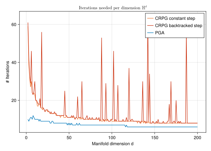

CairoMakie.Screen{IMAGE}

and the number of iterations reads

fig2 = Figure()
axis2 = Axis(fig2[1, 1]; title=L"\text{Iterations needed per dimension }$\mathbb{H}^d$")
lines!(axis2, n_range, [bi[:CRPG_CN][:Iter] for bi in b]; label="CRPG constant step", color=tol_vibrant[1])
lines!(axis2, n_range, [bi[:CRPG_BT][:Iter] for bi in b]; label="CRPG backtracked step", color=tol_vibrant[5],)
lines!(axis2, n_range, [bi[:PGA][:Iter] for bi in b]; label="PGA", color=tol_vibrant[2],)
axis2.xlabel = "Manifold dimension d"
axis2.ylabel = "# Iterations"
axislegend(axis2; position=:rt)

Makie.Legend()

display(fig2)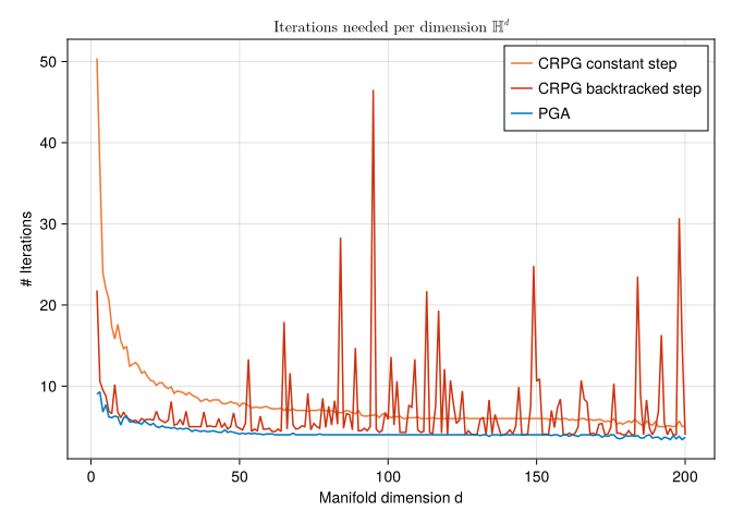

CairoMakie.Screen{IMAGE}

Literature

[BFNZ25]: R. Bergmann, O. P. Ferreira, S. Z. Németh and J. Zhu. On projection mappings and the gradient projection method on hyperbolic space forms, arXiv preprint (2025).
[BJJP25a]: R. Bergmann, H. Jasa, P. J. John and M. Pfeffer. The Intrinsic Riemannian Proximal Gradient Method for Convex Optimization, preprint (2025), arXiv:2507.16055.

Technical details

This tutorial is cached. It was last run on the following package versions.

Status `~/Repositories/Julia/ManoptExamples.jl/examples/Project.toml`
  [6e4b80f9] BenchmarkTools v1.8.0
  [336ed68f] CSV v0.10.16
  [13f3f980] CairoMakie v0.15.13
  [0ca39b1e] Chairmarks v1.3.1
  [35d6a980] ColorSchemes v3.31.0
  [5ae59095] Colors v0.13.1
  [a93c6f00] DataFrames v1.8.2
  [31c24e10] Distributions v0.25.129
  [e9467ef8] GLMakie v0.13.13
  [5c1252a2] GeometryBasics v0.5.11
  [4d00f742] GeometryTypes v0.8.5
  [7073ff75] IJulia v1.34.4
  [682c06a0] JSON v1.6.1
  [8ac3fa9e] LRUCache v1.6.2
  [b964fa9f] LaTeXStrings v1.4.0
  [d3d80556] LineSearches v7.7.1
  [ee78f7c6] Makie v0.24.13
  [7351309b] ManifoldAsymptote v0.1.0
  [af67fdf4] ManifoldDiff v0.4.5
  [9d80ff41] ManifoldMakie v0.1.2
  [1cead3c2] Manifolds v0.11.28
  [3362f125] ManifoldsBase v2.5.0
⌃ [0fc0a36d] Manopt v0.6.2
  [5b8d5e80] ManoptExamples v0.1.20 `..`
  [51fcb6bd] NamedColors v0.2.3
  [6fe1bfb0] OffsetArrays v1.17.0
  [91a5bcdd] Plots v1.41.6
  [08abe8d2] PrettyTables v3.4.2
  [6099a3de] PythonCall v0.9.35
  [f468eda6] QuadraticModels v0.9.16
  [731186ca] RecursiveArrayTools v4.3.4
  [1e40b3f8] RipQP v0.7.0
Info Packages marked with ⌃ have new versions available and may be upgradable.

This tutorial was last rendered July 21, 2026, 12:44:31.