norm(M::AbstractManifold, A::AbstractAtlas, i, a, Xc)Calculate norm on manifold M at point with parameters a in chart i of an AbstractAtlas A of vector with coefficients Xc in induced basis.
AbstractAtlas{𝔽}An abstract class for atlases with charts that have values in the vector space 𝔽ⁿ for some value of n.
affine_connection!(M::AbstractManifold, Zc, A::AbstractAtlas, i, a, Xc, Yc)Calculate the affine connection on manifold M at point with parameters a in chart i of an AbstractAtlas A of vectors with coefficients Xc and Yc in induced basis and save the result in Zc.
check_chart_switch(M::AbstractManifold, A::AbstractAtlas, i, a)Determine whether chart should be switched when an operation in chart i from an AbstractAtlas A reaches parameters a in that chart.
get_chart_index(M::AbstractManifold, A::AbstractAtlas, i, a)Select a chart from an AbstractAtlas A for manifold M that is suitable for representing the neighborhood of point with parametrization a in chart i.
get_chart_index(M::AbstractManifold, A::AbstractAtlas, p)Select a chart from an AbstractAtlas A for manifold M that is suitable for representing the neighborhood of point p.
get_parameters(M::AbstractManifold, A::AbstractAtlas, i, p)Calculate parameters (local coordinates) of point p on manifold M in chart from an AbstractAtlas A at index i.
induced_basis(::AbstractManifold, A::AbstractAtlas, i, VST::VectorSpaceType = TangentSpaceType())Get the basis induced by chart with index i from an AbstractAtlas A of vector space of type vs. Returns an object of type InducedBasis.
kretschmann_scalar(M::AbstractManifold, A::AbstractAtlas, i, a; backend::AbstractADType = AutoForwardDiff())Compute the Kretschmann scalar at the point given by coordinates a in chart i of atlas A on manifold M.
levi_civita_affine_connection!(M::AbstractManifold, Zc, A::AbstractAtlas, i, a, Xc, Yc; backend::AbstractADType = AutoForwardDiff())Compute the Levi-Civita affine connection on the manifold M at a point with parameters a in chart i of an AbstractAtlas A.
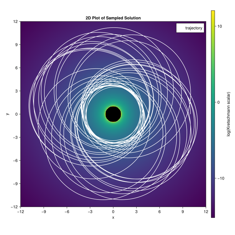
solve_chart_exp_ode(
    M::AbstractManifold, a, Xc, A::AbstractAtlas, i0;
    solver=AutoVern9(Rodas5P()),
    final_time::Real=1.0,
    check_chart_switch_kwargs=NamedTuple(),
    kwargs...,
)
Solve geodesic ODE on a manifold M from point of coordinates a in chart i0 from an AbstractAtlas A in direction of coordinates Xc in the induced basis.
inner(M::AbstractManifold, A::AbstractAtlas, i, a, Xc, Yc)Calculate inner product on manifold M at point with parameters a in chart i of an atlas A of vectors with coefficients Xc and Yc in induced basis.
get_coordinates(M::CenteredMatrices, p, X, ::DefaultOrthonormalBasis{ℝ})Compute the coordinates of in the Euclidean space of matrices, where is the Helmert submatrix, see [Gen17, Section 8.8.1].
manifold_dimension(M::CenteredMatrices)Return the manifold dimension of the CenteredMatrices m-by-n matrix M over the number system 𝔽, i.e.
log(M::CholeskySpace, p, q)Compute the logarithmic map on the CholeskySpace M for the geodesic emanating from the lower triangular matrix with positive diagonal p towards q.
manifold_dimension(M::CholeskySpace)Return the manifold dimension for the CholeskySpace M, i.e.
representation_size(M::CholeskySpace)Return the representation size for the CholeskySpace{N} M, i.e. (N,N).
log(M::Circle, p, q)Compute the logarithmic map on the Circle M.
get_coordinates(M::Circle{ℂ}, p, X, B::DefaultOrthonormalBasis)Return tangent vector coordinates in the Lie algebra of the Circle.
inner(M::Circle, p, X, Y)Compute the inner product of the two tangent vectors X,Y from the tangent plane at p on the Circle M using the restriction of the metric from the embedding, i.e.
manifold_dimension(M::Circle)Return the dimension of the Circle M, i.e. .
manifold_dimension(M::DeterminantOneMatrices{n,𝔽})Return the dimension of the DeterminantOneMatrices matrix M over the number system 𝔽.
manifold_dimension(M::Elliptope)returns the dimension of Elliptope M , i.e.
representation_size(M::Elliptope)Return the size of an array representing an element on the Elliptope manifold M, i.e. , the size of such factor of on .
get_coordinates(M::EssentialManifold, p, X, ::DefaultOrthonormalBasis)
get_coordinates!(M::EssentialManifold, c, p, X, ::DefaultOrthonormalBasis)
Compute the five coordinates of the horizontal tangent vector X at p in an orthonormal basis of the horizontal space.
manifold_dimension(M::EssentialManifold)Return the manifold dimension of the EssentialManifold, which is 5[TD17].
log(M::Euclidean, p, q)Compute the logarithmic map on the Euclidean M from p to q, which in this case is just
norm(M::Euclidean, p, X, r::Real=2)Compute the norm of a tangent vector X at p on the Euclidean M, i.e. since every tangent space can be identified with M itself in this case, just the (Frobenius) norm of X.
inner(M::Euclidean, p, X, Y)Compute the inner product on the Euclidean M, which is just the inner product on the real-valued or complex valued vector space of arrays (or tensors) of size , i.e.
manifold_dimension(M::Euclidean)Return the manifold dimension of the Euclidean M, i.e. the product of all array dimensions and the real_dimension of the underlying number system.
representation_size(M::Euclidean)Return the array dimensions required to represent an element on the Euclidean M, i.e. the vector of all array dimensions.
manifold_dimension(M::FixedRankMatrices)Return the manifold dimension for the 𝔽-valued FixedRankMatrices M of dimension mxn of rank k, namely
representation_size(M::FixedRankMatrices)Return the element size of a point on the FixedRankMatrices M, i.e. the size of matrices on this manifold .
manifold_dimension(M::Flag)Return dimension of flag manifold .
log(M::GeneralizedGrassmann, p, q)Compute the logarithmic map on the GeneralizedGrassmann M , i.e. the tangent vector X whose corresponding geodesic starting from p reaches q after time 1 on M.
manifold_dimension(M::GeneralizedGrassmann)Return the dimension of the GeneralizedGrassmann(n,k,𝔽) manifold M, i.e.
representation_size(M::GeneralizedGrassmann)Return the representation size or matrix dimension of a point on the GeneralizedGrassmann M, i.e. for both the real-valued and the complex value case.
manifold_dimension(M::GeneralizedStiefel)Return the dimension of the GeneralizedStiefel manifold M=.
log(M::Rotations, p, q)Compute the logarithmic map on the Rotations manifold M which is given by
get_coordinates(M::Rotations, p, X)
get_coordinates(M::OrthogonalMatrices, p, X)
get_coordinates(M::UnitaryMatrices, p, X)
Extract the unique tangent vector components at point p on Rotations from the matrix representation X of the tangent vector.
get_coordinates(M::UnitaryMatrices, p, X, B::DefaultOrthonormalBasis)Extract the unique tangent vector coordinates at point p on UnitaryMatrices from the skew-Hermitian tangent vector X.
manifold_dimension(M::Rotations)
manifold_dimension(M::OrthogonalMatrices)
Return the dimension of the manifold orthogonal matrices and of the manifold of rotations
manifold_dimension(M::SpecialUnitaryMatrices)Return the dimension of the manifold of special unitary matrices.
manifold_dimension(M::UnitaryMatrices{n,ℂ}) where {n}Return the dimension of the manifold unitary matrices.
manifold_dimension(M::UnitaryMatrices{<:Any,ℍ})Return the dimension of the manifold unitary matrices.
manifold_dimension(N::GraphManifold{𝔽,G,TM,EdgeManifold})returns the manifold dimension of the GraphManifold N on the edges of a graph , i.e.
manifold_dimension(N::GraphManifold{𝔽,G,TM,VertexManifold})returns the manifold dimension of the GraphManifold N on the vertices of a graph , i.e.
log(M::Grassmann, p, q)Compute the logarithmic map on the Grassmann M , i.e. the tangent vector X whose corresponding geodesic starting from p reaches q after time 1 on M.
norm(M::Grassmann, p::ProjectorPoint, X::ProjectorTangentVector)Compute the norm of a ProjectorTangentVector X at p on the Grassmann manifold M.
affine_connection!(M::Grassmann, Zc, A::GrassmannAtlas, i, a, Xc, Yc)Store the Levi-Civita covariant derivative of Yc in direction Xc in Zc, using the standard GrassmannAtlas.
get_chart_index(M::Grassmann, A::GrassmannAtlas, p)
get_chart_index(M::Grassmann, A::GrassmannAtlas, i, a)
Return a chart index suitable for a point p or coordinates a in chart i.
get_parameters!(M::Grassmann, a, A::GrassmannAtlas, i, p)Store the standard affine coordinates of p in a for the chart indexed by the row tuple i.
get_point!(M::Grassmann, p, A::GrassmannAtlas, i::AbstractVector, a)Store in p the point represented by affine coordinates a in the chart of the standard GrassmannAtlas indexed by i.
get_coordinates(M::Grassmann{ℝ}, p, X, B::DefaultOrthonormalBasis)Given a point p on the Grassmann manifold M in Stiefel representation, i.e. compute the coordinates representing the tangent vector X with respect to the DefaultOrthonormalBasis.
inner(M::Grassmann, A::GrassmannAtlas, i::AbstractVector, a, Xc, Yc)Compute the Riemannian inner product of coordinate vectors Xc and Yc at coordinates a in the chart i of the standard GrassmannAtlas.
manifold_dimension(M::Grassmann)Return the dimension of the Grassmann(n,k,𝔽) manifold M, i.e.
representation_size(M::Grassmann)Return the representation size or matrix dimension of a point on the Grassmann M, i.e. for both the real-valued and the complex value case.
manifold_dimension(M::HamiltonianMatrices)Return the dimension of the HamiltonianMatrices M over the number system 𝔽, that is
get_coordinates(M::HeisenbergMatrices, p, X, ::DefaultOrthonormalBasis{ℝ,TangentSpaceType})Get coordinates of tangent vector X at point p from the HeisenbergMatrices M.
manifold_dimension(M::HeisenbergMatrices)Return the dimension of HeisenbergMatrices(n), which is equal to .
log(M::Hyperbolic, p, q)Compute the logarithmic map on the Hyperbolic space , the tangent vector representing the geodesic starting from p reaches q after time 1.
get_coordinates(M::Hyperbolic, p, X, ::DefaultOrthonormalBasis)Compute the coordinates of the vector X with respect to an orthonormal basis of the tangent space at p.
manifold_dimension(M::Hyperbolic)Return the dimension of the hyperbolic space manifold , i.e. .
log(M::Hyperrectangle, p, q)Compute the logarithmic map on the Hyperrectangle M from p to q, which in this case is just
norm(M::Hyperrectangle, p, X, r::Real = 2)Compute the norm of a tangent vector X at p on the Hyperrectangle M, i.e. since every tangent space can be identified with M itself in this case, just the (Frobenius) norm of X.
manifold_dimension(M::Hyperrectangle)Return the manifold dimension of the Hyperrectangle M, i.e. the product of all array dimensions.
representation_size(M::Hyperrectangle)Return the array dimensions required to represent an element on the Hyperrectangle M, i.e. the vector of all array dimensions.
manifold_dimension(M::InvertibleMatrices{n,𝔽})Return the dimension of the InvertibleMatrices matrix M over the number system 𝔽, which is the same dimension as its embedding, the Euclidean(n, n; field=𝔽).
manifold_dimension(M::MultinomialDoubleStochastic)returns the dimension of the MultinomialDoubleStochastic manifold namely
representation_size(M::AbstractMultinomialDoublyStochastic)return the representation size of doubly stochastic matrices, which are embedded in the matrices and hence the answer here is .
manifold_dimension(M::MultinomialSymmetric)returns the dimension of the MultinomialSymmetric manifold namely
manifold_dimension(M::MultinomialSymmetricPositiveDefinite)Return the dimension of the MultinomialSymmetricPositiveDefinite manifold,
affine_connection!(M::ParametricSurface, Zc, A::ParametricSurfaceAtlas, i, a, Xc, Yc)Store the Levi-Civita affine connection in forwarded chart coordinates in Zc.
check_chart_switch(M::ParametricSurface, A::ParametricSurfaceAtlas, i, a; kwargs...)Delegate the chart-switch condition to the parameter-space atlas wrapped by A.
get_chart_index(M::ParametricSurface, A::ParametricSurfaceAtlas, i, a)Return the chart index in A containing the point represented by local coordinates a in chart i.
get_chart_index(M::ParametricSurface, A::ParametricSurfaceAtlas, p)Return the chart index in A containing embedded point p.
get_parameters!(M::ParametricSurface, a, A::ParametricSurfaceAtlas, i, p)Store in a the local parameters of embedded point p in chart i of ParametricSurfaceAtlas A.
get_point!(M::ParametricSurface, p, A::ParametricSurfaceAtlas, i, a)Store in p the embedded point represented by local parameters a in chart i of ParametricSurfaceAtlas A.
inner(M::ParametricSurface, A::ParametricSurfaceAtlas, i, a, Xc, Yc)Return the pullback Euclidean inner product of chart-coordinate vectors Xc and Yc.
manifold_dimension(M::ParametricSurface)Return the dimension of the parameter space of M.
representation_size(M::ParametricSurface)Return the representation size of the Euclidean embedding of M.
get_coordinates(::PositiveNumbers, p, X, ::DefaultOrthonormalBasis{ℝ})Compute the coordinate of vector X which is tangent to p on the PositiveNumbers manifold.
inner(M::PositiveNumbers, p, X, Y)Compute the inner product of the two tangent vectors X,Y from the tangent plane at p on the PositiveNumbers M, i.e.
manifold_dimension(M::PositiveNumbers)Return the dimension of the PositiveNumbers M, i.e. of the 1-dimensional hyperbolic space,
log(M::ProbabilitySimplex, p, q)Compute the logarithmic map of p and q on the ProbabilitySimplex M.
manifold_dimension(M::ProbabilitySimplex)Returns the manifold dimension of the probability simplex in , i.e.
representation_size(::ProbabilitySimplex)Return the representation size of points in the -dimensional probability simplex, i.e. an array size of (n+1,).
get_coordinates(M::AbstractProjectiveSpace, p, X, B::DefaultOrthonormalBasis{ℝ})Represent the tangent vector at point from the AbstractProjectiveSpace in an orthonormal basis.
manifold_dimension(M::AbstractProjectiveSpace{𝔽}) where {𝔽}Return the real dimension of the AbstractProjectiveSpace M, respectively i.e. the real dimension of the embedding minus the real dimension of the field 𝔽.
representation_size(M::AbstractProjectiveSpace)Return the size points on the AbstractProjectiveSpace M are represented as, i.e., the representation size of the embedding.
log(M::MetricManifold{ℝ, Segre{ℝ,V}, WarpedMetric{A}}, p, q)Logarithmic map on the warped Segre manifold.
log(M::Segre{ℝ, V}, p, q)Logarithmic map on the Segre manifold.
get_coordinates(M::Segre{𝔽, V}, p, X, ::DefaultOrthonormalBasis)Get coordinates of X in the tangent space using a DefaultOrthonormalBasis on each factor.
get_coordinates(
    M::MetricManifold{𝔽, Segre{𝔽, V}, WarpedMetric{A}}, p, X, ::DefaultOrthonormalBasis
)
Get coordinates of X in the tangent space using a DefaultOrthonormalBasis on each factor.
get_coordinates(M::KendallsPreShapeSpace, p, X, ::DefaultOrthonormalBasis)Compute the coordinates of the tangent vector X at p on the KendallsPreShapeSpace M in an orthonormal basis.
manifold_dimension(M::KendallsPreShapeSpace)Return the dimension of the KendallsPreShapeSpace manifold M.
manifold_dimension(M::KendallsShapeSpace)Return the dimension of the KendallsShapeSpace manifold M.
manifold_dimension(M::SkewHermitianMatrices)Return the dimension of the SkewHermitianMatrices matrix M over the number system 𝔽, i.e.
manifold_dimension(M::Spectrahedron)returns the dimension of Spectrahedron M, i.e.
representation_size(M::Spectrahedron)Return the size of an array representing an element on the Spectrahedron manifold M, i.e. , the size of such factor of on .
log(M::AbstractSphere, p, q)Compute the logarithmic map on the AbstractSphere M, i.e. the tangent vector, whose geodesic starting from p reaches q after time 1.
affine_connection!(M::Sphere, Zc, A::StereographicAtlas, i, a, Xc, Yc)Store in Zc the covariant derivative of the coordinate vector field Yc in the coordinate direction Xc at stereographic coordinates a in chart i of A.
get_chart_index(M::Sphere, A::StereographicAtlas, p)
get_chart_index(M::Sphere, A::StereographicAtlas, i, a)
Return the preferred chart index for a point p on M, or for coordinates a in chart i.
get_parameters!(M::Sphere, x, A::StereographicAtlas, i, p)Store in x the stereographic coordinates of the point p in chart i of A.
get_point!(M::Sphere, p, A::StereographicAtlas, i, x)Store in p the point on M represented by stereographic coordinates x in chart i of A.
get_coordinates(M::AbstractSphere{ℝ}, p, X, B::DefaultOrthonormalBasis)Represent the tangent vector X at point p from the AbstractSphere M in an orthonormal basis by rotating the hyperplane containing X to a hyperplane whose normal is the -axis.
manifold_dimension(M::AbstractSphere)Return the dimension of the AbstractSphere M, respectively i.e. the dimension of the embedding -1.
representation_size(M::AbstractSphere)Return the size points on the AbstractSphere M are represented as, i.e., the representation size of the embedding.
manifold_dimension(M::SphereSymmetricMatrices{𝔽})Return the manifold dimension of the SphereSymmetricMatrices n-by-n symmetric matrix M of unit Frobenius norm over the number system 𝔽, i.e.
get_chart_index(M::Stiefel, A::StiefelAtlas, p)Return a Cayley chart centered at p, using the lexicographically first row minor with maximal absolute determinant.
get_parameters!(M::Stiefel, a, A::StiefelAtlas, i::StiefelChart, p)Store the Cayley coordinates of p in the chart centered at i.center.
get_point!(M::Stiefel, p, A::StiefelAtlas, i::StiefelChart, a)Store in p the point represented by Cayley coordinates a in chart i.
manifold_dimension(M::Stiefel)Return the dimension of the Stiefel manifold M=.
representation_size(M::Stiefel)Returns the representation size of the Stiefel M=, i.e. (n,k), which is the matrix dimensions.
manifold_dimension(M::SymmetricMatrices{n,𝔽})Return the dimension of the SymmetricMatrices matrix M over the number system 𝔽, i.e.
log(M::MetricManifold{ℝ,<:SymmetricPositiveDefinite,LogCholeskyMetric}, p, q)Compute the logarithmic map on SymmetricPositiveDefinite M with respect to the LogCholeskyMetric emanating from p to q.
log(M::SymmetricPositiveDefinite, p, q)
log(M::MetricManifold{SymmetricPositiveDefinite,AffineInvariantMetric}, p, q)
Compute the logarithmic map from p to q on the SymmetricPositiveDefinite as a MetricManifold with AffineInvariantMetric.
manifold_dimension(M::SymmetricPositiveDefinite)returns the dimension of SymmetricPositiveDefinite M , i.e.
representation_size(M::SymmetricPositiveDefinite)Return the size of an array representing an element on the SymmetricPositiveDefinite manifold M, i.e. , the size of such a symmetric positive definite matrix on .
manifold_dimension(M::SymmetricPositiveSemidefiniteFixedRank)Return the dimension of the SymmetricPositiveSemidefiniteFixedRank matrix M over the number system 𝔽, i.e.
manifold_dimension(::SymplecticMatrices)Returns the dimension of the symplectic manifold embedded in , i.e.
manifold_dimension(::SymplecticGrassmann)Return the dimension of the SymplecticGrassmann(2n,2k), which is
manifold_dimension(::SymplecticStiefel)Returns the dimension of the symplectic Stiefel manifold embedded in , i.e. [BZ21]
check_chart_switch(::EmbeddedTorus, A::DefaultTorusAtlas, i, a; ϵ = pi/3)Return true if parameters a lie closer than ϵ to chart boundary.
inner(M::EmbeddedTorus, ::DefaultTorusAtlas, i, a, Xc, Yc)Inner product on EmbeddedTorus in chart i in the DefaultTorusAtlas. between vectors with coordinates Xc and Yc tangent at point with parameters a.
manifold_dimension(M::EmbeddedTorus)Return the dimension of the EmbeddedTorus M that is 2.
manifold_dimension(::Tucker)The dimension of the manifold of tensors of multilinear rank , i.e.
get_coordinates(M::Veronese, p, X, ::DefaultOrthonormalBasis; kwargs...)Get coordinates of in using a DefaultOrthonormalBasis.
manifold_dimension(M::Veronese)For M = Veronese(N, D), return the manifold dimension .
solve_chart_exp_ode(
    M::AbstractManifold, a, Xc, A::AbstractAtlas, i0;
    solver=AutoVern9(Rodas5P()),
    final_time::Real=1.0,
    check_chart_switch_kwargs=NamedTuple(),
    kwargs...,
)
Solve geodesic ODE on a manifold M from point of coordinates a in chart i0 from an AbstractAtlas A in direction of coordinates Xc in the induced basis.